|
Monte Carlo Simulation |
|
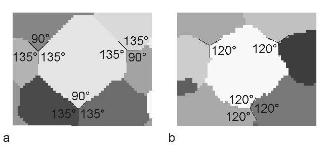
Monte Carlo methods were originally practiced under the name statistical sampling. The credit for inventing the Monte Carlo method is often given to Stanislaw Marcin Ulam (1909-1984), who worked with John von Neumann on the United States’ Manhattan Project during World War II. The most widely known discovery is his design of the hydrogen bomb together with Edward Teller in 1951. But he also ‘invented’ the Monte Carlo method in 1946 while trying to estimate the chances to win the card game Patience. In the following years (1946-1949) Ulam worked together with John von Neumann and Nicholas Metropolis with the aim to develop algorithms for computer implementations and to investigate transformations of non-random problems into random algorithms. It was finally Metropolis who named the new method after the casinos of Monte Carlo. The method itself, however, is much older. The first application has been reported from the year 1777, where the French naturalist Georges-Louis Leclerc, Comte de Buffon (1707-1788) invited this method to approximate Pi with 3.1. This first application is today called Buffon’s needle experiment. The original application of this method in physics comes from solid states physics, where it has been used to model ferromagnetic materials. The magnetization is represented by spins, which can have two possible states: up or down. This kind of model is called Ising model [Ising (1925)]. Already in 1952 [Potts (1952)] generalised the Ising model allowing Q-states for each spin. For this reason the model is called Q-states Potts model or more precisely Q-states Ising model. Today a large field of application is the mesoscopic simulation of materials, especially the simulation of recrystallization and grain growth. In 1984 Anderson et al. for the first time introduced the Potts model to simulate the grain growth kinetics and to investigate grain size distribution and topology in two dimensions [Anderson et al. (1984); Srolovitz et al. (1984)]. They extended the algorithm 1989 to investigate also three-dimensional grain growth [Anderson et al. (1989)]. A recent overview on the Monte Carlo Potts model algorithm for single phase normal grain growth with improved accuracy and efficiency is given by [Yu and Esche (2003a)]. Today there is a growing range of publications in the field of simulation and theory of normal grain growth in three dimensions based on the Potts model algorithm (cf. e.g. [Song and Liu (1998a); Hui et al. (2003); Yu and Esche (2003b); Zöllner and Streitenberger (2004); Zöllner and Streitenberger (2005); Huang et al. (2006)] and the literature within). Further publications concerning the simulation of abnormal grain growth, oriented and anisotropic grain growth and the simulation of two phase materials can also be found. Preparation of the simulation: Before starting the simulation the continuously given microstructure has to be mapped on to a discrete lattice, and one has to decide what lattice and boundary condition to take. In 2D simulations a quadratic lattice with eight nearest neighbours or a triangular one with six nearest neighbours are often used. Although the quadratic lattice is the simplest one to implement, there has been a discussion throughout the years, if this underlying lattice forces the simulation results. Figure 1 shows this point of discussion. In Figure 1a a graphical representation of a simulated 2D grain structure with simulation temperature 0 is shown. One can see that the grain boundaries cling to the underlying lattice and triple points where three grains meet do not have the 120° angles as expected for normal grain growth. The reason of these effects is substantiated in the Monte Carlo Potts model method itself. It simulates curvature driven grain growth, where the system energy is minimized by decreasing the boundary length. That is why the driving force places the grain boundaries along lattice facets, which results in a clinging of grain boundaries to the underlying lattice. Because these lattice effects are strictly depending on the simulation algorithm and therefore highly non-physical, one has to eliminate them from the simulation. Holm et al. (1991) have shown two practical possibilities to do so:
 Figure 1: a - Clinging of grain boundaries to the lattice at temperature 0; b - grain boundaries with 120° angles in equilibrium at high simulation temperature. On the other hand the triangular or hexagonal lattice already intrinsically yields the 120° equilibrium angles at simulation temperature 0. But again the grain boundaries cling to the lattice, although one can’t see it. Therefore, it is here also useful to increase the simulation temperature. In three dimensions a cubic lattice is mostly chosen with 26 nearest neighbours including the first nearest neighbours with the Euclidian distance l from the centre lattice point, the second nearest neighbours and the third nearest neighbours. Each lattice point represents in the simulation a so called Monte Carlo unit (MCU), which has assigned a crystallographic orientation specified by the rotation angles in the three-dimensional Euler space. Furthermore, the boundary condition can be chosen either as fixed, as free or as periodic. The most common one is the periodic boundary condition, where in three dimensions the leftmost lattice plane connects from the right side to the rightmost lattice plane, the foremost connects to the hindmost and the undermost connects to the topmost. The advantages of this condition are:
A fixed boundary condition means that all MCUs on the boundary of the lattice do not change their properties during the simulation. Basic Monte Carlo Potts model algorithm: The smallest time unit of the Monte Carlo Potts model simulation is called one Monte Carlo step (MCS) and defined as N reorientation attempts, where N is equal to the total number of MCUs of the lattice. That means, a 3D simulations with a lattice of size 200 × 200 × 200 has a total number of reorientation attempts equal to N = 8,000,000. Each reorientation attempt itself consists of the following steps:
|
| [Ising (1925)] | E. Ising. Beitrag zur Theorie des Ferromagnetismus. Zeitschrift für Physik, 31:253, 1925. |
| [Potts (1952)] | R.B. Potts. Some generalized order-disorder transformations. Proceedings of the Cambridge Philosophical Society, 48:106, 1952. |
| [Anderson et al. (1984)] | M.P. Anderson, D.J. Srolovitz, G.S. Grest, and P.S. Sahni. Computer simulation of grain growth - 1. Kinetics. Acta Metallurgica, 32:784, 1984. |
| [Srolovitz et al. (1984)] | D.J. Srolovitz, M.P. Anderson, P.S. Sahni, and G.S. Grest. Computer simulation of grain growth - 2. Grain size distribution, topology and local dynamics. Acta Metallurgica, 32:793, 1984. |
| [Anderson et al. (1989)] | M.P. Anderson, G.S. Grest, and D.J. Srolovitz. Computer simulation of normal grain growth in three dimensions. Philosophical Magazine B, 59:293, 1989. |
| [Yu and Esche (2003a)] | Q. Yu and S.K. Esche. A Monte Carlo algorithm for single phase normal grain growth with improved accuracy and efficiency. Computational Materials Science, 27:259, 2003a. |
| [Song and Liu (1998a)] | X. Song and G. Liu. A simple and efficient three-dimensional Monte Carlo simulation of grain growth. Scripta Materialia, 38:1691, 1998a. |
| [Hui et al. (2003)] | L. Hui, W. Guanghou, D. Feng, B. Xiufang, and F. Pederiva. Monte Carlo simulation of three-dimensional polycrystalline material. Materials Science and Engineering: A, 357:153, 2003. |
| [Yu and Esche (2003b)] | Q. Yu and S.K. Esche. Three-dimensional grain growth modeling with a Monte Carlo algorithm. Materials Letters, 57:4622, 2003b. |
| [Huang et al. (2006)] | C. Ming Huang, C.L. Joanne, B.S.V. Patnaik, and R. Jayaganthan. Monte Carlo simulation of grain growth in polycrystalline materials. Applied Surface Science, 252:3997, 2006. |
| [Holm et al. (1991)] | E.A. Holm, J.A. Glazier, D. Srolovitz, and G.S. Grest. The effect of lattice anisotropy and temperature on grain growth in the two-dimensional Potts model. Physical Review A, 43:2662, 1991. |
| [Read and Shockley (1950)] | T.W. Read and W. Shockley. Dislocation models of crystal grain boundaries. Physical Review, 78:275, 1950. |
| [Humphreys (1997)] | F.J. Humphreys. A unified theory of recovery, recrystallization and grain growth, based on the stability and growth of cellular microstructures - I. the basic model. Acta Materialia, 45:4231, 1997. |
| [Huang and Humphreys (2000)] | Y. Huang and F.J. Humphreys. Subgrain growth and low angle boundary mobility in aluminum crystals of orientation {110}<001>. Acta Materialia, 48:2017, 2000. |
| [Zöllner and Streitenberger (2004)] | D. Zöllner and P. Streitenberger. Computer simulations and statistical theory of normal grain growth in two and three dimensions. In Recrystallization and grain growth, B. Bacroix et al. editors, volume 467-470, page 1129, Trans Tech Publications, 2004. |
| [Zöllner and Streitenberger (2005)] | D. Zöllner and P. Streitenberger. Monte Carlo simulation of grain growth in three dimensions. In Continuous Casting, H.R. Müller editor, page 168, Weinheim, Wiley-VCH, 2005. |
| [Zöllner and Streitenberger (2008)] | D. Zöllner and P. Streitenberger. Normal grain growth: Monte Carlo Potts model simulation and mean-field theory. In Micro-Macro-Interactions in Structured Media and Particle Systems, A. Bertram and J. Tomas, editors, page 3, Springer Verlag, 2008. |
| [Zöllner (2006)] | D. Zöllner. Monte Carlo Potts Model Simulation and Statistical Mean-Field Theory of Normal Grain Growth. Shaker-Verlag, Aachen, 2006. |
Datenschutzerklärung der Otto-von-Guericke-Universität Magdeburg nach DSGVO

 .
.
